Lesson 5: Google sheets

Lesson Outline

Today let's get focused on spreadsheets.

Spreadsheets

After the lesson the students should know what a spreadsheet is and what are the their key concepts

Setup

Make sure all the laptops are either plugged or with the battery full enough to last for 1 hour at least. Try to set every laptop in the same place as the previous class.

Instructor’s laptop is connected to the projector or big screen.

Do the attendance!

Content

Recap

Do a quick recap of what was explained last day. Get focused on formatting the text again, and undoing changes. And again, make sure they are getting better using track-pad.

Google sheets

What they are?

A spreadsheet (google sheets are a flavor of Spreadsheet as Excel is), is a tool to handle data in a tabular way.

A sheet is composed of rows and columns. And in each intersection of a row and a column there is a cell. And a Cell is where the data is stored.

Moving around the sheet

Before starting adding data, give some time to the students to get used to the sheet format itself.

Show them how to, or better ask them to try to, select a cell (single click) , move to contiguous cells (arrow keys), select more than one cell (press shift and click on several contiguous cells), etc…

Then show them how to change the background color of a cell or group of cells.

Adding data

Now we are ready to start adding data. For instance you can start by creating a very simple table to store the list of students, with their name, surname and age (or any other field that comes to your mind).

4 or 5 students must be more than enough.

Once the table is done, explain again how to highlight the first row (header) by changing background color, centering the text and making it bold.

List of countries in European Union

As they already know how to build a table, now you can ask them to create a list of countries in the European Union. For each country we want to store:

• Name

• Capital

• Population

• Link to wikipedia

So they can start by adding the header of the table. And of course they should search the list of members using google. And once they get the list, they should pick 4 countries and add them to the table.

So once the 4 countries are chosen, they should now search one by one to find Capital and population.

Most likely they will end up in Wikipedia after first search. At this point you can remind them that there are two ways to keep searching all the remaining countries. Google (general search) or inside Wikipedia.

This exercise is going to keep them busy for a while. Try to notice if a student got stuck and guide him or her to the next step.

Merging data

Once everyone is done, ask the to share the data of one of the countries they added to the list with you, and write each one in your own sheet in different rows.

This is just a previous step to explain can be done in a way better way: by sharing the document among us all.

Renaming and adding sheets

Let's start with something easy. Show the students how to rename a sheet and how to add a new one

Sharing same sheet

In order to get all the students working in the same document, ask them to share their emails with you.

Give them access to a new empty google sheet in your own folder.

At this moment explain a bit further what sharing documents means:

By default when a document is added to a folder in Drive, only the owner of the document can access it. But what google drive is really good at is sharing content. So by sharing a specific document or folder, we are making a piece of our file system (Drive) accessible to a group of known users.

We can share documents as read only or in edit mode as well.

Also there are two ways of sharing the document.

• By providing the list of users we want to share the document with

• Or generating a link and sending this link to our contacts

First option is always better and safer. Explain to them why… or as usual, try to push for them to guess the reason.

Editing the document all together

The students should now go to Gmail (remember they can get there with the google apps button), and open the new email which is given them access to the shared file.

Click on the link.

When everyone is in the file, add a header for the list of countries with:

• Name

• Capital

• Population

• Area

Now share your screen and assign every student two rows of the shared sheet (assuming header is in row 2, student A takes rows 3 and 4, student B 5 and 6 and so on).

Ask them to fill the rows with the data they have in their own sheet. Only the first 3 columns, as the Area is new.

While editing the file in their own computer, they will see how things are also changing in your shared screen.

When all the rows are filled up, now ask them to look for the area of each country, but to make it collaborative, each student will search the Area of the countries added by another student (student A takes now rows 5 and 6, student B 7 and 8 and so on)

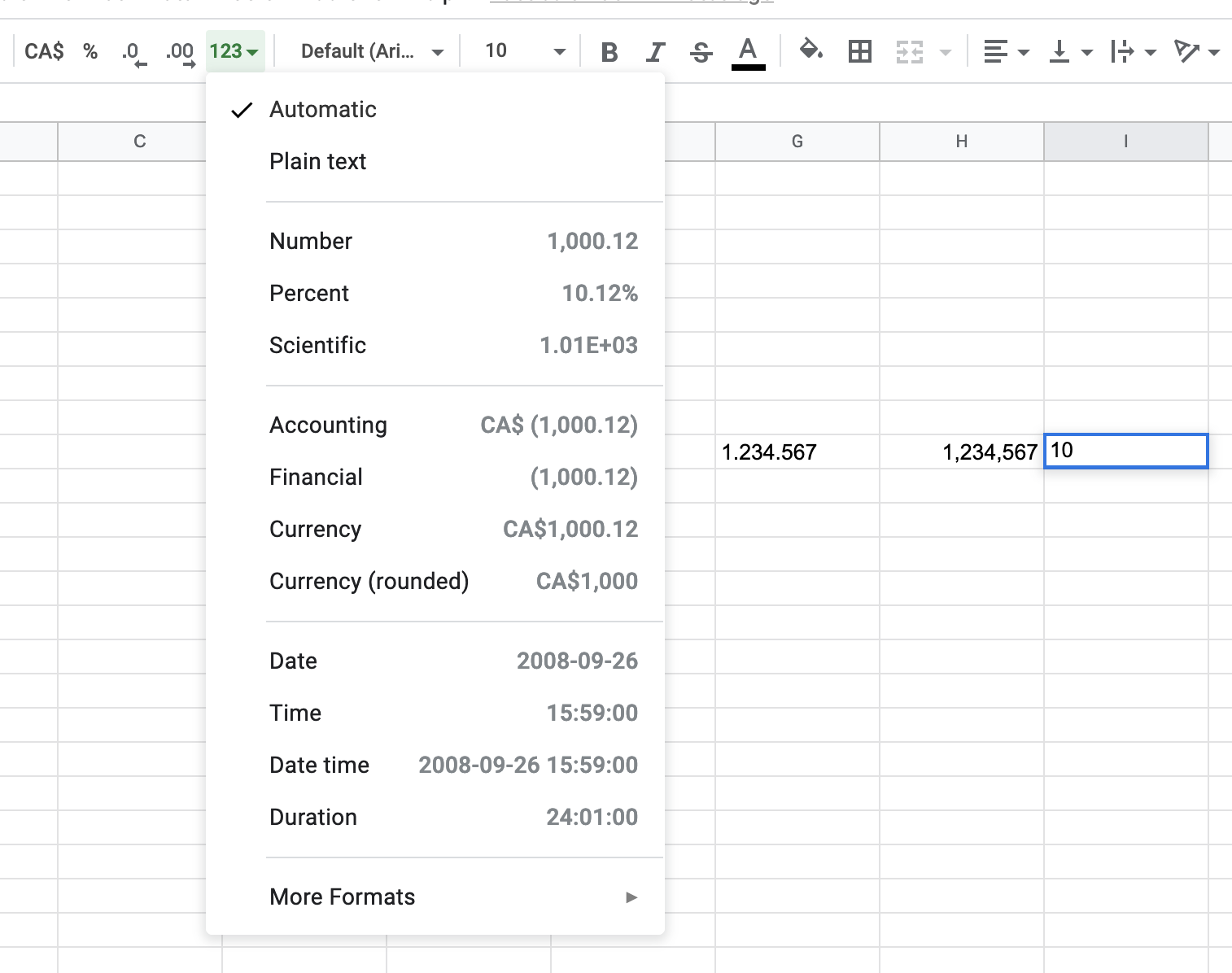
Cell type

Show them how to set the type of data in a cell. Google sheet itself is setting the type of a cell based on its content. Mainly text and numbers.

But as users we can explicitly let google sheets know what kind of data is stored in a cell:

• Plain text

• Number without decimals

• Number one ore more decimals

• Currency

• Percentage

• etc

Functions

Show them now how to add a function to a cell. Type 3 or four number in consecutive cells, from top to bottom. Use easy number:)

And then select the cell at the bottom of last number and start typing the formula in the content box:

Hit enter so that the additions of all the numbers will show.

Of course to show how good is this feature, change the value of one or several numbers for the to see how the SUM gets automatically updated.

Note here that this is a big step for them. At leat the group I was teaching got a bit confused about this crazy thing called Functions.

So might be good spending some time going to the differnt tables, and repeat the steps on their computers step by step.

More Formulas

As said at the end of previous lesson, the students got a bit confused with formulas. So let's start again from scratch.

SUM

Repeat the SUM function by adding several numbers in several contiguous cells, and in the last one add the sum function.

Once done, show them again how changing one of the numbers make the SUM result to change as well.

Now repeat all the steps, but this time select the range of cells with the cursor. Type =SUM( in the function's box, then move the cursor to first cell, click on it, press shift, click on the last cell and hit enter.

Ask them to repeat the steps. Try to check if all of them are doing it, as they might struggle a bit with the combination of track-pad and Shift key.

Now change one of the numbers with a text, and show them how the text is ignored in the result of the sum.

Arithmetic

Add two number 2 one after another in two different columns. In the next column at the right, declare the arithmetic sum function using + operand. Something like =B1+C1

And then keep adding other arithmetic operations like subtract, multiply or divide.

Concatenation

Now, using the shared sheet, ask them to write their name in a cell, and their surname in the next column. Assign a row to each student.

Write also your own name and surname.

Once all the names and surnames are written, concatenate your name and surname using CONCATENATE function.

Exercise - Build a Logical Test in Excel

What it a logical test

Logical tests are everywhere.

• Is my salary higher than my colleague's?

• Is my rent higher than my neighbor's?

• Is the quantity in stock larger now than at the beginning of the month?

• Does a ticket is closed or not?

• ...

A logical test is just a comparison between 2 items.

Construction of a logical test

You can create a logical test in a cell WITHOUT using the IF function.

In fact, it is the opposite. A test is used in an IF function.

A test in Excel is very simple.

1. Start your test with the equals sign =.

2. Then add a value or cell reference

3. Then the logical symbol (see below)

4. Then another cell or another value

For instance, write the following formula in a cell to see the result

=C2="Closed"

Logical symbols you can use

To create a test, you can use one of the following symbol

• = equal to

• > greater than

• >= greater than or equal to

• < lower than

• <= lower or equal to

• <> not equal to

Examples of logical tests

On the previous example, we have created a test with the string "Closed". But you can build a test with numerical values or formulas

Example 1: Does the age is greater than 21?

If you want to know if the cell contents are greater than a specific value, like 21, you can write the following test.

=B2>21

Example 2: Compare 2 cells

You can also create the same test but this time, the value 21 is in the cell G4. So, instead of comparing one cell with one value, you can also create a test between 2 cells

=B2>=$G$4

In this example, we must add dollars to block the reference of the cell G4

Example 3: Is the cell empty or not?

Now, if you want to know if a cell is not empty, you will write the following formula

=A2<>""

The 2 double quotes is the code for an empty cell (it's a string with nothing in between)

Many functions return TRUE or FALSE

Excel has a collection of functions that return TRUE or FALSE. These functions start with IS

• ISBLANK

• ISERROR

• ISFORMULA

• ISNA

• ISNUMBER

• ISNONTEXT

For instance, a common mistake in Excel is to write the month in letter instead of customize your date format. So, because a date is a number in Excel, we can create this test to check if a cell contents a date or not.

=ISNUMBER(B2)

Function COUNTIF

A basic task with Excel is to count the number of rows for a specific criteria. The function COUNTIF do that easily

Presentation of COUNTIF

The function COUNTIF counts the number of rows for one criteria.

The function requires only two arguments

• The range of cells where is your data

• The value you search (the criterion).

=COUNTIF(Range of cells, criteria of selection)

Example with COUNTIF

In the following document, you have a list of sales.

You want to know how many times you have sold Banana.

To return the number of time you have the name Banana in your list, you have to write the formula like this

=COUNTIF(B3:B12,"Banana")

And the result is

Replace the criteria by a cell reference

Now if instead of typing the name of the data you want to have the reference of a cell where its value = the name you want

For instance, you can use the cell G4 where its value is Banana

=COUNTIF(B3:B12,G4)

Not sensitive case

Don't worry if your criteria hasn't the same case of the data in your table, the function COUNTIF, is not sensitive case.

For instance, in this example, we want to count the number of times we have the word PEACH in uppercase and the result is